Michele Andreolli, Paolo Surico
What is the consumption response to unexpected transitory income gains of different size and what are the aggregate demand implications of stimulus packages that target different segments of the population? This column explores these questions using responses to hypothetical questions in the Italian Survey of Household Income and Wealth. Families with low cash-at-hand display a higher marginal propensity to consume out of small gains, while affluent households exhibit a higher marginal propensity to consume out of large gains. For a given level of public spending, a fiscal transfer of a smaller size paid to a larger group of low-income households stimulates aggregate consumption more than a larger transfer paid to a smaller group.
The global pandemic of 2020–21 has attracted renewed attention to how fiscal policy can support aggregate demand and stimulate consumer spending. For instance, the recent $1.9 trillion Biden plan in the US comprises $1 trillion of direct transfer to households, with about 40% of it targeted to financially vulnerable groups. In order to understand the effects of this fiscal plan on aggregate demand, it is crucial to identify how a household’s marginal propensity to consume (MPC) is related to the size of the stimulus payments a household receives and how this MPC varies along the income distribution.
If, on the one hand, the MPC was small – with the windfall mostly used to save or repay debt (Mian and Sufi 2010, Romer 2021) – and invariant to income, then large and untargeted fiscal transfers would be needed to generate a significant boost to aggregate consumption. If, on the other hand, the MPC was higher for smaller payments to low-income families, then less sizeable but targeted transfers could have an even larger aggregate demand impact, and at a significantly lower cost for public finances.
Unfortunately, the empirical evidence is at best scant on how the MPC for temporary windfalls varies jointly with the size of the shock and the level of household resources. An inherent limitation of existing studies is that households typically receive only one stimulus payment, rather than two payments of significantly different sizes. Therefore, identifying the MPC for small and large shocks necessarily relies on comparing households with different characteristics.
This is problematic for two reasons. First, the size of any actual fiscal transfer is endogenous and dependent on observed characteristics such as income, job status, marital status, and number of children. Second, households may also differ along unobserved characteristics, which would make it hard to interpret any MPC heterogeneity as the result of mere heterogeneity in the shock size.
MPC heterogeneity in 3D: Across shock size, household resources, and non-essential budget shares
In a recent paper (Andreolli and Surico 2021), we overcome these important limitations by comparing the MPC for small and large income gains for the very same household. We do so by exploiting a unique set of questions in the Italian Survey of Household Income and Wealth, which ask respondents how much they would spend in response to a one-off increase in their disposable resources as large as one month’s and one year’s worth of their income, respectively.
The advantage of this approach is twofold. First, by focusing on within-household variation only, one can be confident that any MPC heterogeneity does not reflect unobserved heterogeneity. Second, the difference in the magnitude of the two income gains is not only independent of individual characteristics but also sufficiently large to elicit any possible heterogeneity in spending due to the size of the windfall.
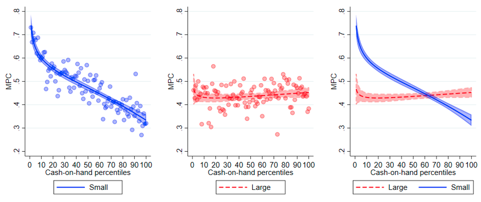
Figure 1 shows our key findings. In the left panel, we plot the average MPC response to a one-month shock by each cash-on-hand percentile, where cash-on-hand is the sum of disposable income and financial assets. We fit a fractional polynomial on the percentile bins and plot the 95% confidence intervals as well. The central panel shows the plot with the MPC response to a large shock. The right panel overlaps the non-parametric estimates of the relationship between MPC and cash-on-hand for the two shock sizes.
Figure 1 The distribution of MPC by cash-on-hand percentiles for small income gains (in blue) and large income gains (in red)

Notes: The plot shows the MPC by each cash-on-hand percentile in 2010 and fits a fractional polynomial with 95% confidence bands based on the percentile bins. The first panel plots the MPC out of a small gain, the second one out of a large gain. The third one plots both fractional polynomials together. Cash-on-hand is the sum of disposable income and financial assets.
Two key results stand out. First, the MPC for small income changes is a negative function of household resources, whereas the MPC for large income changes displays a slightly positive gradient. Second, families with low cash-on-hand exhibit a higher MPC for the smaller gains, whereas affluent households are characterised by a higher MPC for the larger windfalls.
The behaviour of poorer households is consistent with the presence of uninsurable income risk and borrowing constraints: large shocks are more likely to help households overcome the liquidity constraint and therefore lower the MPC. On the other hand, the behaviour of more affluent households is not easily rationalised by this class of models.
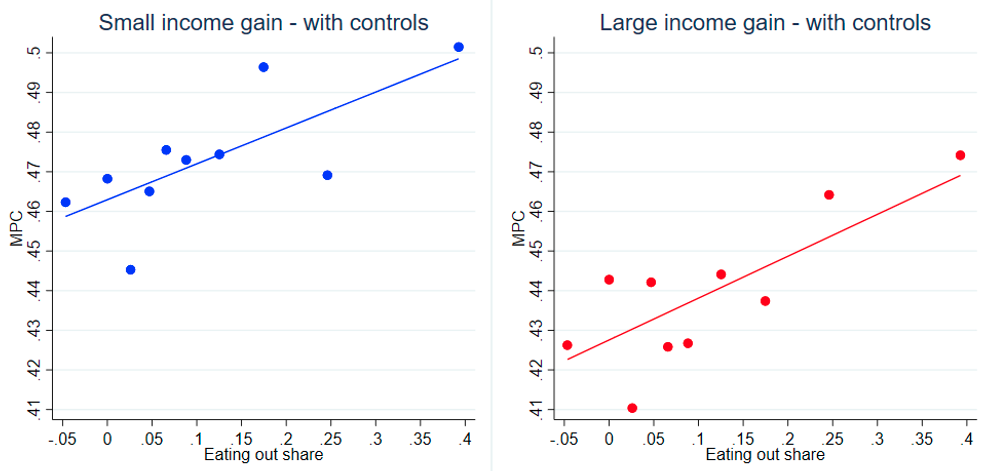
In order to explore the consumption behaviour of families at the top of the cash-on-hand distribution, we examine the role of non-homotheticity in consumption baskets. Affluent households devote a significantly larger share of their food spending on eating out, which we interpret as a proxy for the importance of non-essential goods and services in their consumption basket. In Figure 2, we relate the budget share spent on luxury goods to the two MPC measures reported in Figure 1. Figure 2 reveals that, after controlling for liquid wealth, a higher share of non-necessity consumption predicts a higher MPC for both small and large income gains.
Figure 2 MPC and non-essential spending

Notes: In this plot, we relate eating-out share (the share of food expenditures made outside the home over total food expenditures, measured in 2012) with different measures of the MPC. The two plots show the result from a binned scatter plot on the MPC out of a small gain (first panel) and out a large shock (second panel). Both panels control for cash-on-hand deciles and demographic characteristics. All controls are demeaned and are measured in 2010. Demographic controls are: age in[18,30], age in[30,45], age in[45,60], male, married, years of education, family size, resident in the South, unemployed, and the real log change in household cash-on-hand between 2012 and 2010. Only households who are present in both years are included. The lines are OLS regression lines.
Our favourite interpretation of the MPC heterogeneity in Figure 1, supported by the suggestive evidence in Figure 2, is that borrowing constraints are a significant determinant of spending among households with low cash-on-hand. Therefore, these may be responsible for the empirical finding that the MPC for small income gains is higher than for large gains at the bottom of the income distribution. Among affluent households, however, liquidity considerations are likely less salient and non-essential items are a far stronger driver of expenditure. Non-homothetic preferences may thus provide a rationale for the empirical result that families with high cash-on-hand exhibit a higher MPC for large income gains.
To evaluate this conjecture, we derive the predictions of a model with non-homothetic preferences on non-essential consumption and show that, in sharp contrast to the model with borrowing constraints and idiosyncratic risk, it can account for both our new empirical findings. First, MPC and disposable resources from the large income gains are positively correlated at the household level; second, affluent families exhibit a higher MPC for the larger windfalls. The intuition is that non-homothetic preferences imply that non-necessities spending is easier to postpone (or anticipate) than essential purchases. Moreover, the price of non-necessities tends to increase faster than the price of necessities over time.
In summary, a model with non-homothetic preferences across consumption goods generates two predictions: (i) the MPC is increasing in income; and (ii) among households with a large share of non-essential spending, namely high earners, the MPC for large gains is higher than for small gains. These predictions are consistent with an increasing number of empirical analyses that report significant MPCs also among high-income households (e.g. Misra and Surico 2014, Kueng 2018, Chetty et al. 2021).
Our empirical and theoretical findings therefore extend in a novel dimension the contribution of existing empirical studies. Such studies, while well suited to document heterogeneity across household resources (e.g. Johnson et al. 2006, Jappelli and Pistaferrri 2010), cannot typically investigate within-household heterogeneity across shock size.
Targeted fiscal policies
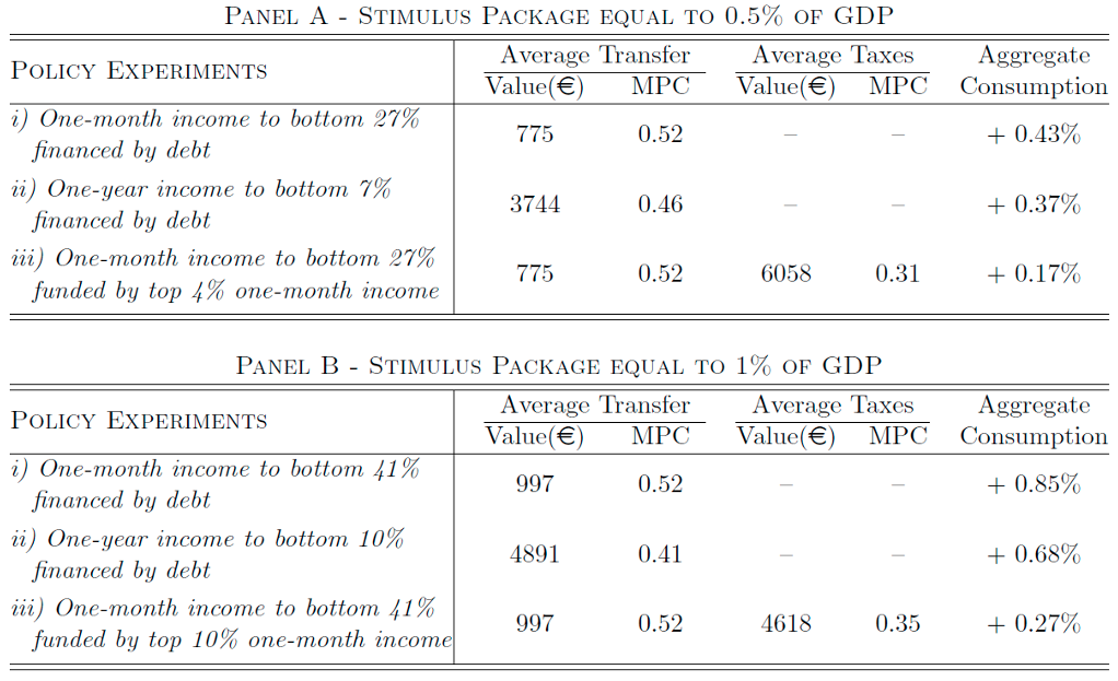
As for policy implications, we simulate several fiscal experiments that vary either the size of the transfer to households or how the stimulus package is financed. We consider fiscal stimulus packages of two sizes, equal to 0.5% and 1% of GDP, respectively. The top panel of Table 1 presents the case of a stimulus package as large as 0.5% of GDP. The first row – policy (i) – reveals that a package of this size would allow the government to pay one month of income to the bottom 27%, for an average transfer value of €775 in the second column. As households in this group exhibit an average MPC of 0.52 (out of the small income gain) and the economic stimulus payment is financed by debt, the last column indicates that policy (i) would boost aggregate consumption by 0.43%.
In the second row, we consider an alternative policy that uses a 0.5% of GDP stimulus package to pay one year of income to the bottom 7% of the cash-on-hand distribution, for an average transfer of €3,744 among these 7% families. Policy (ii), which is also financed by debt, has a smaller effect on aggregate consumption than policy (i), around 0.37%. The reason is that (as the third column shows) policy (ii) is associated with a lower average MPC of 0.46 (out of the large income gain).
A similar result is seen in the second panel of Table 1, about a 1% of GDP stimulus package. Policy (i), with one month of income to the bottom 41%, stimulates aggregate demand more than policy (ii), with one year of income, at 0.85% versus 0.68%, respectively.
Table 1 Fiscal experiments

Notes: The aggregate stimulus-package amount is constant in each panel. In the first and second rows of each panel, the transfer increase is financed by an increase in debt to GDP. The aggregate increase in tax revenues in the third row of each panel is, by construction, as large as the increase in debt to GDP under the debt financing scenarios. In the first and third (second) rows of each panel, the transfer is equal to one month (year) of income for the households at the bottom of the cash-on-hand distribution as indicated in the first column. The average amount of the transfer is specified in the second column, and the average MPC resulting from this transfer is specified in the third column. In the third row of each panel, the tax disbursement is equal to one month of income for households at the top of the cash-on-hand distribution, as indicated in the first column. The average tax payment is presented in the fourth column, and the resulting average MPC is in the fifth column. All variables are weighted by the population weights to be representative of the Italian population. Cash-on-hand is the sum of disposable income and financial assets. In the first and second rows of each panel, the change in aggregate consumption is computed as the ratio between the sum of the spending increases by the households who received a transfer and the level of total aggregate consumption by all households. In the third row of each panel, the change in aggregate consumption is net, as the (negative) change in spending for the households who paid more taxes is subtracted from the (positive) change in spending for the households who received a transfer.
The second result from this experiment comes from inspecting a tax finance scenario. The third row of panel A considers a policy that is all like policy (i) except that the stimulus package is now funded by a tax increase for the top 4% as large as one month of their income, for an average disbursement of €6,058.1 As policy (iii) is funded by raising taxes rather than debt, it is not surprising that it has a smaller aggregate impact. Yet, because of the significant gap between the average MPCs at each end of the cash-on-hand distribution (i.e. 0.52 for transfers in the third column versus 0.31 for taxes in the fifth column), policy (iii) would provide a significant stimulus to aggregate consumption, around 0.17%, but with no increase in government debt.
A similar result is seen in panel B with a 1% of GDP stimulus package. Tax finance yields still a positive net effect on aggregate consumption, of 0.27%, as poorer households exhibit a higher MPC than richer households.
In summary, these fiscal experiments suggest a simple policy lesson: less is more. An economic stimulus payment of smaller size and targeted to a larger share of disadvantaged families would provide a stronger boost to aggregate consumption than a larger transfer paid to a smaller share of poorer households. While debt-financed interventions are associated with the largest aggregate impact, a fiscal policy that redistributes resources from the top to the bottom of the income distribution would deliver an economically significant stimulus to the aggregate economy at no additional cost for public finances.
References
Andreolli, M, and P Surico (2021), “Less is more: Consumer spending and the size of economic stimulus payments”, CEPR Discussion Paper 15918.
Chetty, R, J Friedman and M Stepner (2021), “Effects of January 2021 stimulus payments on consumer spending”, Opportunity Insights Economic Tracker.
Christelis, D, D Georgarakos, T Jappelli, L Pistaferri and M van Rooij (2019), “Asymmetric consumption effects of transitory income shocks”, Economic Journal 129(622): 2322–41.
Jappelli, T, and L Pistaferri (2010), “The consumption response to income changes”, Annual Review of Economics 2: 479–506.
Johnson, D, J A Parker and N Souleles (2006), “Household expenditure and the income tax rebates of 2001”, American Economic Review 96: 1589–610.
Kueng, L (2018), “Excess sensitivity of high-income consumers”, The Quarterly Journal of Economics 133(4): 1693–751.
Mian, A, and A Sufi (2010), “Household leverage and the recession of 2007–09”, IMF Economic Review 58(1): 74–117.
Misra, K, and P Surico (2014), “Consumption, income changes and heterogeneity: Evidence from two fiscal stimulus programmes”, American Economic Journal: Macroeconomics 6(4): 84–106.
Romer, C D (2021), “The fiscal policy response to the pandemic”, Brookings Papers on Economic Activity.
Source: https://voxeu.org/article/smaller-economic-stimulus-payments-could-boost-consumer-spending-more


